Neural network classification of countries in the OECD

In the previous couple of posts I discussed the application of both regression (estimation of a continuous output for a given input sample) and classification (estimation of the class to which a given input sample belongs) machine learning methods with application to socio-economic data. Specifically multi-dimensional linear regression was used to estimate the average life expectancy for a particular country from a series of continuous socio-economic factors. Logistic regression was also used to classify if a country belonged to the OECD or not in a particular year. Here I will illustrate a way to build predictive classification models using artificial neural networks (ANN) machine learning algorithms.

The formulation of ANNs is inspired by the structure of the brain. They are represented as a network of interconnected neurons, and are used to learn both regression and classification functions from data samples comprising of potentially a large number of input variables. This general approach has produced state-of-the-art results in computer vision, speech recognition and natural language processing [1,2,3]. ANNs are also referred to as feed-forward neural network, multi-layer perception, and more recently deep networks/learning. Deep learning has come to represent applications in which the amount of feature engineering is minimised, with the machine learning tasks achieved through multiple learned layers of neurons. Each neuron undertakes a weighted sum over a series of inputs then applies a nonlinear activation function producing an output value, as illustrated below. For regression problems the rectified linear unit (ReLU) is a popular activation function. For classification problems the sigmoid or hyperbolic tangent functions as used in logistic regression are the most common activations functions.

The input variables in a ANN are introduced into an input layer. These inputs are fed into a hidden layer of neurons. The outputs from the first hidden layer may then be fed into a second hidden layer. There may well be many hidden layers, with each layer learning more complex and more specialised behaviour. The penultimate hidden layer feeds its outputs to the final output layer. This typical structure of an ANN is illustrated below. Each circle represents a neuron, and the lines represent the interconnections. For a given network, the credit assignment path (CAP) is the path of nonlinear functions from an input to the output. The length of the CAP for a feed-forward neural network is the number of hidden layers plus one for the output layer. In recurrent neural networks a signal may pass through a given layer on multiple occasions, which means the length of the CAP is unbounded.

The weights in each neuron are learnt from the training data, such that they minimise a specified cost function. The cost function comprises of a loss (or error) function element that quantifies the difference between the value estimated by the ANN and the true value. For regression problems one would use a least squares error measure, whilst for classification problems a log-likelihood (or information entropy) measure is more appropriate. The cost function may also contain some additional regularisation terms which specify the relative importance put on minimising the amplitude of the model weights.

In ANNs the cost function is typically minimised using the back-propagation method. In the standard back-propagation method the weights are updated using some form of convex optimisation method, such as the gradient decent algorithm. In the gradient decent algorithm one first calculates the gradient/derivative of (change in) the cost function with respect to the weights, with the gradient averaged across all samples in the training set. The value of each weight from the previous iteration is then updated by adding to it the cost function gradient multiplied by a specified constant rate of learning. Here I adopt the mini-batch stochastic gradient descent variant, where the cost function gradient is averaged over only a small batch of samples in the training set, as opposed to all of the available samples. The larger the batch size the better the estimate of the gradient, but the more time taken to calculate the gradient. The batch size that returns the model coefficients with the least amount of computational resources is problem dependent, but typically ranges in order from 1 to 100 [4]. A very good explanation and illustration of the back-propagation method and gradient decent algorithm can be found in [5].

There are various frameworks available for creating ANN applications including:

• Theano is a python library developed at University of Montreal, which calculates the partial derivatives required for the back-propagation algorithm using symbolic mathematics [4,6,7].
• Torch is a deep learning framework developed using the Lua programming language, and is currently being co-developed and maintained by researchers at facebook, google deepmind, twitter and New York University.
• DeepLearning4J is an open-source, parallel deep-learning library for Java and Scala, which can be integrated with Hadoop and Spark databases management systems.
• Caffe is a C++ deep learning framework developed at Berkeley University with python and matlab interfaces.

As an illustration I have repeated the OECD classification problem solved in the previous blog post using logistic regression. To briefly recap the goal is to build a classification model determining if a particular country in a particular year is in the OECD on the basis of various socio-economic measures including: GDP; average life expectancy; average years spent in school; population growth; and money spent on health care amongst others. Here the classification problem is solved using a ANN with 12 input variables, one hidden layer comprising of 24 neurons, all of which feeding into one output neuron. A hyperbolic tangent activation function is used for the hidden layer neurons, and a sigmoid activation function for the output neuron. The model weights are randomly initialised using a uniform probability distribution. The code is written in python using the theano library.

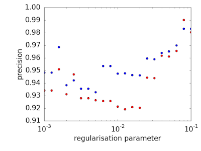
The ANN is calculated over the training data set using L2 regularisation, with the regularisation parameters ranging from 0.001 and 0.1. The predictive performance measures of precision (P = [True positive] / [True positive + False positive], recall (R = [True positive] / [True positive + False negative]) and F1 score (2P*R/(P+R)) are calculated for each regularisation parameter over the training and validation data sets and illustrated in the following figures. As expected each performance measure of is greater for training data set than the validation data set across most regularisation levels.

The ANN with the greatest F1 score over the validation data set has a regularisation level of 0.001. The learning curves illustrating the F1 curve as a function of the number of samples used to train this particular model is illustrated below. The fact that the learning curves of the training and validation data sets do not converge indicate that the predictive performance could be further improved with additional data.

One final note, ANNs are biologically inspired learning algorithms, but the mathematical form of the neurons is far simpler than the behaviour of biological neurons. There are a range of methods that aim to more closely replicate the learning processes in the brain. The human brain actually consists of several levels (of which neurons are only one), each of which serve a slightly different purpose in the learning process [8]. Algorithms that attempt to replicate this process are refereed to as cortical learning algorithms.

References:

[1] http://yann.lecun.com/exdb/mnist/

[2] Deng, L.; Li, Xiao (2013). "Machine Learning Paradigms for Speech Recognition: An Overview". IEEE Transactions on Audio, Speech, and Language Processing.

[3] Socher, Richard (2013). "Recursive Deep Models for Semantic Compositionality Over a Sentiment Treebank"
[4] LISA lab (2015), "Deep Learning Tutorial", University of Montreal.

[5] https://class.coursera.org/ml-005/lecture

[6] F. Bastien, P. Lamblin, R. Pascanu, J. Bergstra, I. Goodfellow, A. Bergeron, N. Bouchard, D. Warde-Farley and Y. Bengio. “Theano: new features and speed improvements”. NIPS 2012 deep learning workshop.

[7] J. Bergstra, O. Breuleux, F. Bastien, P. Lamblin, R. Pascanu, G. Desjardins, J. Turian, D. Warde-Farley and Y. Bengio. “Theano: A CPU and GPU Math Expression Compiler”. Proceedings of the Python for Scientific Computing Conference (SciPy) 2010. June 30 - July 3, Austin, TX

[8] https://www.youtube.com/watch?v=6ufPpZDmPKA

Supervised machine learning – classification of countries in the OECD

To recap from the previous post supervised machine learning aims to build predictive models linking a series of inputs to a series of outputs, as opposed to unsupervised machine learning which builds descriptive models representing the data at hand. There are two types of supervised machine learning: regression, that predicts a continuous number for a given input sample; and classification that predicts to which class (or group) a particular sample belongs. Here we will be concentrating on classification.

In the previous post, I built a regression model predicting the average life expectancy of a country from various socio-economic input factors. As an example of classification, I will use this same data set to determine if a particular country in a particular year is in the OECD (that is the group of countries belonging to the Organisation for Economic Co-operation and Development) or not. The list of input factors/fields (with the associated variable name in parentheses) include: 

• Life expectancy (lifeExp)
• GDP per capita (gdpPC)
• Total per capita spend on health (healthPC)
• Government per capita spend on health (healthPCGov)
• Births per capita (birth)
• Deaths per capita (death)
• Deaths of children under 5 years of age per capita (deathU5)
• Years women spend in school (womenSchool)
• Years men spend in school (menSchool)
• Population growth rate (popGrowth)
• Population (pop)
• Immigration rate (immigration)
• Flag stating whether a country in a particular year is the OECD (oecd).

The data was downloaded from the Gapminder and OECD websites, data wrangling was done using pandas, machine learning undertaken using scikit-learn, and visualisations developed using matplotlib and seaborn.

For clarity I have visualised the data for the key factors determined in the previous regression study against the OECD flag variable. If a country in a particular year is in the OECD the variable is given a value of oecd=1, if it is not in the OECD is has a value of oecd=0. Let us first consider the subplot below highlighted by the black box, which is the per capita death rate of children under the age of 5 (deathU5) versus the OECD flag. One can see that only countries with a low infant death rate are in the OECD, however, there are also certain countries with low infant death rates that are not in the OECD. By inspecting the remaining subplots one can also say that in general countries in the OECD have higher life expectancies, lower birth rates and spend more money on health care. The supervised machine learning task is to use these inputs fields (and the others listed above, but not visualised here) to predict whether or not a particular country in a particular year is in the OECD.

There are various classification algorithms that one could use including: logistic regression; support vector machines (also known as large margin classifiers); k-nearest neighbours; or neural networks / deep learning (the subject of the following post). In this example I will be adopting logistic regression [1], which essentially aims to fit to the data an "S" shaped curve, called the sigmoid" (or logistic) function, as opposed to the linear function used in the previous regression example. The inputs to the sigmoid function are again the feature variables and model parameters, however the output is now bounded by 0 and 1, and can be interpreted as being the probability of a particular sample belonging to the class at hand. In the present example the output is the probability of a country being in the OECD. If the probability is greater than 0.5 then it estimated to be in the OECD, if the probability is less than 0.5 it is estimated to not be in the OECD. In general, however, this threshold of 0.5 can be modified to control the predictive performance of the model.

Before building the model, each of the features are first standardised, by subtracting away the mean and then dividing by the standard deviation. To address underfitting (high bias) and overfitting (high variance) we first break the available data into a training data set (consists of 60% of the samples) to build the model, a cross validation data set (20% of the samples) to select the optimal regularisation level/hyper-parameter, and a test data set (remaining 20% of the samples) to determine the performance of the optimal model. I reduce the complexity of the logistic regression model by applying an L1 regularisation on the model parameters, which penalises candidate models for having large magnitude coefficients, with the penalty proportional to the regularisation hyper-parameter. This concept is discussed further in the previous post with respect to regression. The stronger the regularisation level the more simple the final model, and the weaker the regularisation the more complex the model becomes.

The quantification of the error in classification is not as straight forward as in regression studies, particularly for skewed data in which there may be many more negative samples (not in the OECD) as opposed to positive samples (in the OECD) or vice-versa. In regression studies the cost function is simply the summed squared error between the model prediction and the true value. In classification studies there are four types of prediction outcomes:

• true positive - a positive result (in OECD) is predicted for a positive event (in OECD)
• true negative - a negative result (not in OECD) is predicted for a negative event (not in OECD)
• false positive (or a Type I error) - a positive result (in OECD) is predicted for a negative event (not in OECD)
• false negative (or a Type II error) - a negative result (not in OECD) is predicted for a positive event (in OECD)

Associated with these outcomes are two measures: precision; and recall.

Firstly, precision (P) is the proportion of correctly predicted positive events to the total amount of events predicted as positive (True positives / [True positives + False positives]). The precision versus regularisation level is illustrated in the figure below. For all plots in this post the blue dots represent the training data set, and the red dots the cross validation data set. Typical of machine learning studies, the precision (inversely proportional to the generalisation error) of the training data set is greater than the precision of the cross validation data set for all regularisation levels. As the regularisation level increases the precision of the training data set tends upwards, particularly for very small regularisation levels as the model becomes increasingly complex. This means that the countries that are predicted as being in the OECD are in the OECD the vast majority of the time. 

Recall (R) is the proportion of correctly predicted positive events to the total amount of actual positive events (True positives / [True positives + False negatives]). Typically the greater the precision the lower the recall. We can see from the figure below, for both the training and cross validation data sets as the regularisation level decreases and the model becomes more complex, the recall of the model reduces (as the precision increases). This means that while the countries that are predicted as being in the OECD are in the OECD the vast majority of the time (high precision), the model is also classifying many countries as not being in the OECD when in fact they actually are (low recall). For logistic regression one can also trade off the precision and recall measures against each other by modifying the threshold probability (set to 0.5 here) between positive and negative events. This effect is discussed in more detail in [2].

One way of combining the precision (P) and recall (R) measures of model performance is the F1 score, given by 2*P*R/(P+R). This measure is illustrated below over the same range of regularisation parameters. The optimal model is defined as the one with the highest F1 score in predicting the cross validation data set below. This occurs for a regularisation parameter of 1.3.

The next stage is to generate learning curves to determine the sensitivity of the error of the optimal model to the number of samples used to build the model. If sufficient data has been used to build the model, then the performance measures of the model over the test and cross validation sets should converge. As the number of samples used to build the model increases, the performance measures of the test data set should decrease (generalisation error increase), whilst the performance measures of the cross validation data set should increase (generalisation error decrease). This appears to be the case from the precision learning curve illustrated below. The convergence is less clear, however, when inspecting the associated plots for the recall and F1 score measures.

The dominant model coefficient in the optimal model are associated with the average life expectancy (lifeExp), government spend on health care (healthPCGov) and the infant death rate (deathU5). The ability of the optimal model is found to have an F1 score of approximately 0.9 for the training, cross validation and test data sets. To improve the predictability of the classification model (and also the regression model in the previous post) one could adopt a more complex unsupervised machine learning method, such as neural networks. This will be the subject of the following post.

References:

[1] Cox, D.R., 1958, "The regression analysis of binary sequences", J Roy Stat Soc B, Vol. 20,  215–242.

[2] Ng, A., 2015, Course in Machine Learning, Stanford University, https://class.coursera.org/ml-005/lecture

Supervised machine learning - regression of life expectancy

In this post I will use machine learning to determine the key factors driving life expectancy in the countries of the world throughout history. Firstly, I will provide a definition of machine learning and an overview of the available classes of methods following the descriptions outlined in [1]. In general machine learning algorithms learn a model that either predicts or describes features of a particular system from a series of input (and potentially output) samples, by minimising some error measure (generalisation error). In this context, features are the variables (or dimensions) that describe the system, and a sample is one observation of that system. Typically features would be the columns in a database, and the samples would be the rows.

There are four main machine learning categories:

• Supervised (predictive), in which both inputs and output features are known.
• Semi-supervised (predictive), in which some of the data used to train the models is either noisy or missing.
• Unsupervised (descriptive), in which only the inputs are available.
• Reinforcement (adaptive), where feedback is applied via a series of punishments and rewards based on how well the algorithm performs in a given environment. Feedback control systems are one such example, as discussed in the final chapter of my PhD thesis.

In supervised and semi-supervised machine learning there are only two possible tasks:

• Regression - a continuous number is estimated from the input values. Specific techniques include multi-dimensional linear regression and its variants. Recursive Bayesian Estimation, as discussed in a previous blog post, can be considered as an example of a semi-supervised regression algorithm.
• Classification - a discrete quantity is estimated, determining the class to which a particular sample belongs. For example, determining the species of flower from the length and width of its petals, or voice to text conversion. Specific techniques include logistic regression and support vector classifiers. In semi-supervised classification, several classification functions may need to be learnt to account to different combinations of missing inputs.

In unsupervised learning a new descriptive representation of the input data is sought. There are various possible tasks including:

• Data decomposition / dimension reduction - the data is decomposed into a series of modes comprising of different combinations of the features/variables that can be used in combination to reconstruct each of the samples. Example decompositions include Fourier, wavelet and principle component analysis as discussed in a previous blog post.
• Clustering - define a finite set of classes (or categories) to describe the data. The classes can be determined on the basis of the feature centroids (eg: K-means), assumptions of the data distribution (eg: Gaussian Mixture Models) or on the density of the clustering of the points (eg: mean shift)
• Density estimation – estimates the probability density function (PDF) from which the samples are drawn. Examples methods include: histograms in which the feature dimensions are discretised and samples are binned creating vertical columns; and kernel density estimation in which samples contribute to a Gaussian distribution locally producing a smoother final PDF.
• Anomaly detection – determining which samples in the existing data set are outliers. This can be based on statistics (i.e. how many standard deviations away from the mean), or on the multi-dimensional distance between samples.
• Imputation of missing values – Estimate the missing values in a data set. This can be undertaken by conditioning the PDF on the available values, replacing the missing values with either the mean or median of the existing values, replacing with a random selection from the range of possible values, or interpolating in time between samples for time series data.
• Synthesis and sampling – generate new samples that are similar, but not identical, to the training data set. An example is the generation of initial conditions for ensemble numerical weather prediction.

In the current example we will adopt supervised machine learning (specifically multi-dimensional linear regression) to build a predictive model of life expectancy. Potential key socio-economic factors (with the associated variable name in parentheses) include: 

• Life expectancy (lifeExp)
• GDP per capita (gdpPC)
• Total per capita spend on health (healthPC)
• Government per capita spend on health (healthPCGov)
• Births per capita (birth)
• Deaths per capita (death)
• Deaths of children under 5 years of age per capita (deathU5)
• Years women spend in school (womenSchool)
• Years men spend in school (menSchool)
• Population growth rate (popGrowth)
• Population (pop)
• Immigration rate (immigration)

Each of these features were downloaded from the Gapminder website. The following data mining exercise is undertaken using the python eco-system. The wrangling of the input data was done using pandas, the machine learning tasks undertaken using scikit-learn, and the visualisations developed using matplotlib and seaborn.

The first step is to calculate the correlations between each of the fields to determine likely important factors. In the figure below red indicates features that are strongly positively correlated, blue strongly negatively correlated, and grey weakly correlated. We find that the life expectancy is weakly correlated with population growth, population, and immigration rate. We also find that total health spend per capita, and government health spend per capita are similarly correlated with other fields. Likewise, the number of years spent in school by women and men, are similarly correlated with the other fields.

The next step is to build a regression model linking the life expectancy to the other features. Each feature is first standardised, by subtracting away the mean and then dividing by the standard deviation. When developing any form of model from data it is important to address under and over fitting. Underfitting (high bias) of the data occurs when the learning function is not complex enough to represent the observations. Overfitting (high variance) occurs when the learning function is too complex. We address these aspects by first breaking the available data into the following three sets:

• training data set, typically consists of 60% of the total amount of data available, which is used to first build the model for a given set of fitting parameters;
• cross validation data set, consisting of 20% of the data, over which the error prediction is calculated, with the optimal model parameters determined as the model of minimum error; and
• test data test, consisting of the remaining 20% of the data, which is used to determine the performance of the optimal model.

An excellent discussion on this concept can be found in [3].

I use the LASSO regression method [2] to reduce the complexity of the model as far as possible by regularising the regression coefficients. Regularisation is a means of reducing the capacity / complexity of the learning function. It can be thought of as a mathematical representation of Occam's razor, or the reductionist idea that among equally well performing candidate models, one should select the least complex. The stronger the regularisation level, the greater the tendency to remove features that do not contribute to the improved prediction of the model. The squared error versus regularisation level is illustrated in the figure below. As is typical of machine learning studies, the generalisation error of the training data set decreases as the regularisation parameter decreases, or equivalently as the model becomes more complex. The generalisation error of the cross validation data set initially decreases with increasing complexity and reduced underfitting, until it reaches a minimum error, after which the error increases due to overfitting. To address underfitting (high variance) one can either: increase the regularisation; fit to less features; or get more training data. To address overfitting (high bias) one can either: decrease the regularisation; or fit to more features, including nonlinear combinations of features. The regularisation parameter can be considered as a hyper-parameter, in that it is a parameter that defines how the model is fit to the data, as opposed to the model parameters that define the model itself.

The next stage is to generate learning curves, that is determine the sensitivity of the error of the optimal model to the number of samples used to build the model. As illustrated below, and again typical of machine learning studies, as the number of samples used to build the model increases, the generalisation error of the training set increases as it attempts to represent more observations. At the same time the generalisation error of the cross validation set decreases as the model becomes more representative of reality. An indication that sufficient data has been used to build the model, is when the error measures calculated from the two data sets are equal. The error of the training data set is the lower limit. If this error is deemed too high, additional data will not help the future predictability of the model. In this scenario to improve accuracy one must either reduce the regularisation, add in additional input features, or use more complex regression methods (eg: multi-layer neural networks).

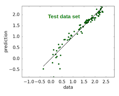
The ability of the model with the lowest squared error to predict the cross validation data set, is then used to predict the test data set, as illustrated below. Each green dot represents a country in a particular year. A perfect model would have all of the points lying along the black line. This model did not use the features of immigration, years women spent in school, and government health spend. The last two features were not required as they are strongly correlated with years men spent in school and total health spend, respectively. In addition the regression coefficients for the features of population, population growth, years men spent in school, GDP and death rate were also orders of magnitude smaller than the coefficients of the dominant features. 

The correlation coefficients of the remaining key features are illustrated below. This indicates that life expectancy is most strongly related to child death rate, with a strong negative correlation of -0.93. This makes sense, since the deaths of very young people would bring down the average life expectancy of the entire country. We also find that the birth rate is higher in countries with higher child death rate, with a strong positive correlation of 0.84. Finally the child death rate is lower in countries with higher health spend per capita, with a negative correlation of -0.4.

When inspecting scatter plots of the key features, the relationship between child death rate and health spend per capita is actually far stronger than the correlation coefficient of -0.4 initially suggests. In the scatter plot highlighted in the figure below you can see there is a very tight arrangement of the samples, with the child death rate dropping rapidly past a threshold health care spend. The relationship is a very strong, but not a linear one, which is why the correlation coefficient was not excessively high. To improve the predictability of the model one could perform a transformation linearising the data prior to undertaking the regression, or adopt a nonlinear regression method such as neural networks. This will be the subject of a future post. For completeness, histogram estimates of the probability density functions are illustrated in the plots along the diagonal of the figure below.

In summary the best way to improve the life expectancy of a country is to reduce the child death rates, which has a very strong relationship to the money spent on health care.

References:

[1] Bengio, Y., Goodfellow, I. J. & Courvill, A., Deep Learning, book in preparation for MIT press, www.iro.umontreal.ca/~bengioy/dlbook

[2] Tibshirani, R. 1996, Regression shrinkage and selection via the lasso, J. Roy. Soc. B., pp267-288.

[3] Ng, A., 2015, Course in Machine Learning, Stanford University, https://class.coursera.org/ml-005/lecture

Calibration of Computationally Expensive Simulations via Response Surface Optimisation

In this post I will provide a general definition of optimisation, and an overview of some popular algorithms. I will then go through an example on the use of response surface optimisation to determine the turbulence model parameters that minimise the error between a computational expensive fluid flow simulation of a submarine, and associated experimental measurements. We first presented this work in [1].

Optimisation is the means of determining the design parameters that minimise a specified cost function, under a set of constraints. For example if we want to minimise the noise of a fan, then the cost function would be the decibel level of the noise generated by the fan, and the design parameters would include the width, length, thickness and material type of the fan blades. There may also be a constraints put on the weight and sharpness of the components for occupational, health and safety reasons. Constraints limit the allowable combination of design parameters, and typically result in a lower performance design had the constraints not been in place. The cost functions can also be multi-objective. For example, in addition to minimising the noise of the fan, one may also want to minimise the time, energy and financial cost required to manufacture the components. Typically the designer must determine the relative importance of each of the objectives to combine them into one cost function.

Optimisation methods can be classed as two different types: gradient based methods; and non-gradient based methods. If the design / parameter space for a given cost function is convex (continually decreasing with only one minimum) then gradient based methods are an extremely efficient way of determining the optimal solution. In these methods one estimates how the cost function changes with the design parameters, and this information is used to select the next combination of parameters to set. However, if the cost functions are not convex and are highly non-linear, then gradient based methods have the potential to get stuck in local minima and produce sub-optimal designs. In this case non-gradient based methods are preferred.

One of the more popular non-gradient based methods is evolutionary optimisation. These methods attempt to evolve an optimal design through natural selection, or survival of the fittest. This is achieved through breeding a set of parents to produce a set of children, and keep only the fittest children (low cost function) for further breeding [2]. Each parent and child have a DNA gene sequence defined by the design input parameters. Breeding is undertaken on the basis of mutation and cross-over (gene swapping). There are two main incarnations that utilise the above approach, genetic algorithms (GA) and evolutionary algorithms (EA). GA were development first, with the parameters encoded into binary numbers, which are essentially treated as genes in the reproductive process. In the mutation process one of the digits in the binary coding is randomly changed from a 1 to a 0 or visa-versa. In the cross-over process to genes are split at a random point and interchanged. EA are philosophically the same, however, the crossover and mutation steps are performed on the design parameters directly, without any binary coding and decoding processes. In either case the breeding process is continued over multiple generations until a sufficiently good solution is found or computational resources are exhausted.

Evolutionary approaches can achieve a very good solution in a reasonable time, however, they require many concurrent evaluations of the cost function [2]. This is not reasonable for cost functions that are very computationally expensive. In this case Response Surface Models (RSM) can be utilised to build an estimate of the parameter space from a limited number of cost function evaluations. The minimum of the RSM is then obtained either numerically or analytically, and the cost function is then re-evaluated for the estimated optimal parameter set. The RSM is updated with the additional cost function evaluation, and the new minimum determined. This process is repeated until there is a sufficiently small difference between the RSM estimate of the cost function minimum and the value obtained from the cost function itself. The only subjective choice is the functional form of the RSM. Popular choices are splines and Kriging [3]. The latter is adopted in the following example. Kriging has the added feature of providing error estimates of the RSM throughout the design space.

As mentioned at the beginning of the post, the optimisation task here is to determine the turbulence model parameters that minimise the error between an expensive computational fluid dynamics (CFD) simulation of a submarine, and associated experimental measurements (lift force, drag force and yaw moment). Slices of the velocity field are illustrated with respect to the submarine body below.

For this particular turbulence model there are two key parameters β_i and α_∞. We, therefore, have a two-dimensional parameter space. Reasonable limits for these two parameters are set, with 9 evenly spaced values are selected along each dimension, producing 9x9=81 design candidates. The CFD simulation was run 81 times - once for each of the design candidates – with the lift force, drag force and yaw moments calculated from the flow field. The multi-objective cost function is the average squared error between the forces calculated from the CFD and the forced measured experimentally. The initial RSM of the simulation error is illustrated below, where blue contours are low error and red contours are high error. The symbols in the figure below represent the initial 81 evaluations of the cost function.

The minimum of this RSM is determined along with the associated values of β_i and α_∞. An additional CFD simulation is run with these particular values of β_i and α_∞. The cost function (error in the forces between the CFD simulation and the measurements) is evaluated and the RSM is updated. This process continues until the difference between the RSM of the cost function and the evaluated cost function is sufficiently small. The final RSM with the additional cost function evaluations are illustrated below.

In addition to determine the optimal solution, the RSM also provides an understanding of how the cost function changes throughout the design space, which evolutionary methods do not. RSM are also capable of answering multiple questions at once. For example in a multi-objective optimisation study if the relative importance of the objectives change, then a new RSM can be built using the existing simulation results. Further refinement of the RSM would in all likelihood be required to find the new optimal solution for the new cost function. If one was to use an evolutionary method, then the optimisation process would have to be run from scratch.

The RSM optimisation method can also be used to determine the optimal hyper-parameters used in the data modelling process, such as regularisation parameters used in regression and classification studies. 

References:

[1] Chng, T. S., Widjaja, R., Kitsios, V. & Ooi , A., RANS Turbulence Model Optimisation based on Surrogate Management Framework , Australasian Fluid Mechanics Conference , Queensland University, Brisbane, Australia , 3-7 December, 2007 .

[2] Fogel, D., 1994, An introduction to simulated evolutionary optimization, IEEE transactions on neural networks, Vol. 5, pp 3-14.

[3] Jones, D. R., 2001, A taxonomy of global optimization methods based on response surfaces, J. Global Opt., Vol. 21, pp 345-383.

Principles of Data Mining and the Scientific Method

This post is intended to serve as an overview of the principles of data mining, and the important stages in the process. Various aspects of these stages will be addressed in detail in future posts.

One can think of data mining as the scientific method re-branded for new a age in which the large volumes of data are available, with additional emphasis placed on the treatment of such data. In the scientific method one observes certain phenomena, and then tests hypotheses proposed to explain these observations (or data sets). In the mature sciences (eg: physics, chemistry) the scientific method has produced rigorous mathematical representations of reality. For example we now know that the acceleration due to gravity (a) acting on an object by another object of much larger mass (M) and radius (R) is a = G M / R², where the gravitational constant is G=6.67384 × 10^-11 m³ kg^-1 s^-2. There is no need to continually re-estimate G from data. Substituting in the mass and radius of the Earth produces a gravitational acceleration of a=9.81ms^-2. However, in many new complex fields including social science, finance, business intelligence and genetics, there are no such fundamental mathematical representations as yet, and one must rely on data mining techniques to build models from the observations in order to make predictions of these systems.

There are six key stages in the data mining process including: 1) pose the question; 2) collect / generate the data; 3) check and clean the data; 4) build and validate the model; 5) use this model to make predictions and/or optimise the system; and 6) report and visualise the results. This process is illustrated below, and is a modified version of that in [1]. The process is illustrated in a sequential manner, but it is in fact iterative. If problems are encountered in downstream stages, then you may have to return to earlier stages to either: build an alternate model; perform additional data checking; collect more data; or pose an alternate question if your original question is inappropriate or unanswerable. I will now provide more details on each of these stages.

It may seem obvious, but the first stage in the process is to pose a question to be answered. Or more specifically pose a hypothesis that can be tested. It is important to be as precise as possible, as this will define the effort and investment required for each of the forthcoming stages in the data mining process. It is also important to do as much background reading on previous work done in the field, as to ensure you are not reinventing the wheel. From my own personal experience, in today's research and commercial environments the problem is typically not that we don't have the sufficient data, but rather we don't have sufficient questions.

The second stage is to collect and store the appropriate type, quality and quantity of data required to answer the question at hand. The data may be collected from observations of the environment (eg: global atmospheric temperature measurements) and/or generated by numerical simulation (eg: general circulation models of the climate). In either case all errors, uncertainties and caveats should be documented.

The third stage involves the collating, checking and cleaning of the data. Aspects that should be checked include:

• Integrate / wrangle the data from various sources into a consistent data structure and check that the data from different sources is in fact consistent.
• Ensure the data has the appropriate type (e.g. integer, float, text, images, video). For example the average number of children per family may be a float (e.g. 2.4) but the number of children in a given family must be an integer (e.g. 2).
• Check that the data is in fact realisable. For example you cannot have a negative amount of rainfall.
• Check that the data is "timely", that is, collected from a period appropriate to answer the question at hand.
• Remove repeated and redundant data.
• Detect and remove outliers / anomalies from the database. This is a large field and will be discussed at a future time.
• Flag samples with any missing values and either remove the entire sample or augment the sample with an appropriate estimate of the missing value. This is also a large field in itself and will be the subject of a future post.

Given that enough storage space is available, it is good practice to keep a copy of the raw data before any checking, cleaning or compression is undertaken. This way if a bug is found in any of the downstream data processing codes, the analysis can be repeated from the source data.

The next phase is to develop models representing the system from which the data was collected. The form of these models is wide and varied and dependent upon the question which you are aiming to answer. For example:

• If you are interested in identifying groups of customers with similar purchasing patterns then clustering methods would be the most appropriate.
• If your project requires image or voice recognition then deep learning methods are at present the optimal solution.
• If you are looking to extrapolate company earnings in a hypothetical future economy then statistical regression may be the most appropriate approach.
• If you need to determine the parameters for models that are very computationally expensive, then one can minimise a response surface model of the simulation error as opposed to the model directly.

I will provide worked examples of each of these applications in future posts. Regardless of the approach it is good practice to build the model using a sub-set of the data (the training set), and verify the model on the remaining data not used during the model training process. If the model does not perform adequately well on the test data, then one may either need to adopt a more complex model, or collect more data, depending on if the model is either under or over fitting the data. This is discussed in more detail in a future post on multi-dimensional linear regression.

Once a model is built and verified it can then be used to make predictions and/or optimise the system design. The most appropriate optimisation method depends on the dimensionality and nonlinearity of the parameter space, and the computational cost required to evaluate the model. Typical available optimisation methods include: gradient base search; genetic algorithms; evolutionary methods; stochastic optimisation; swarm optimisation; and response surface modelling, to name but a few. I will demonstrate the application of response surface models in the following post.

Visualisation of the original data and/or model predictions is an efficient way to report and communicate the results of your analysis. I have already discussed the visualisation of time varying three-dimensional data sets in a previous post. There are also a variety of techniques available for visualising even higher multi-dimensional multi-variate data set. An example would be visualising how the GDP of an economy varies with employment, population, education, water and food availability, etc. There are various techniques available to visualise highly dimensional data sets including: parallel coordinates; radial visualisation; sun burst; and matrix scatter plots.

The following posts will provide further details on the various aspects and facets of data mining highlighted here.

References:

[1] Kantardic, M., 2003, Data mining: concepts, models, methods, and algorithms, Wiley-IEEE Press.