Supervised machine learning - regression of life expectancy

In this post I will use machine learning to determine the key factors driving life expectancy in the countries of the world throughout history. Firstly, I will provide a definition of machine learning and an overview of the available classes of methods following the descriptions outlined in [1]. In general machine learning algorithms learn a model that either predicts or describes features of a particular system from a series of input (and potentially output) samples, by minimising some error measure (generalisation error). In this context, features are the variables (or dimensions) that describe the system, and a sample is one observation of that system. Typically features would be the columns in a database, and the samples would be the rows.

There are four main machine learning categories:

• Supervised (predictive), in which both inputs and output features are known.
• Semi-supervised (predictive), in which some of the data used to train the models is either noisy or missing.
• Unsupervised (descriptive), in which only the inputs are available.
• Reinforcement (adaptive), where feedback is applied via a series of punishments and rewards based on how well the algorithm performs in a given environment. Feedback control systems are one such example, as discussed in the final chapter of my PhD thesis.

In supervised and semi-supervised machine learning there are only two possible tasks:

• Regression - a continuous number is estimated from the input values. Specific techniques include multi-dimensional linear regression and its variants. Recursive Bayesian Estimation, as discussed in a previous blog post, can be considered as an example of a semi-supervised regression algorithm.
• Classification - a discrete quantity is estimated, determining the class to which a particular sample belongs. For example, determining the species of flower from the length and width of its petals, or voice to text conversion. Specific techniques include logistic regression and support vector classifiers. In semi-supervised classification, several classification functions may need to be learnt to account to different combinations of missing inputs.

In unsupervised learning a new descriptive representation of the input data is sought. There are various possible tasks including:

• Data decomposition / dimension reduction - the data is decomposed into a series of modes comprising of different combinations of the features/variables that can be used in combination to reconstruct each of the samples. Example decompositions include Fourier, wavelet and principle component analysis as discussed in a previous blog post.
• Clustering - define a finite set of classes (or categories) to describe the data. The classes can be determined on the basis of the feature centroids (eg: K-means), assumptions of the data distribution (eg: Gaussian Mixture Models) or on the density of the clustering of the points (eg: mean shift)
• Density estimation – estimates the probability density function (PDF) from which the samples are drawn. Examples methods include: histograms in which the feature dimensions are discretised and samples are binned creating vertical columns; and kernel density estimation in which samples contribute to a Gaussian distribution locally producing a smoother final PDF.
• Anomaly detection – determining which samples in the existing data set are outliers. This can be based on statistics (i.e. how many standard deviations away from the mean), or on the multi-dimensional distance between samples.
• Imputation of missing values – Estimate the missing values in a data set. This can be undertaken by conditioning the PDF on the available values, replacing the missing values with either the mean or median of the existing values, replacing with a random selection from the range of possible values, or interpolating in time between samples for time series data.
• Synthesis and sampling – generate new samples that are similar, but not identical, to the training data set. An example is the generation of initial conditions for ensemble numerical weather prediction.

In the current example we will adopt supervised machine learning (specifically multi-dimensional linear regression) to build a predictive model of life expectancy. Potential key socio-economic factors (with the associated variable name in parentheses) include: 

• Life expectancy (lifeExp)
• GDP per capita (gdpPC)
• Total per capita spend on health (healthPC)
• Government per capita spend on health (healthPCGov)
• Births per capita (birth)
• Deaths per capita (death)
• Deaths of children under 5 years of age per capita (deathU5)
• Years women spend in school (womenSchool)
• Years men spend in school (menSchool)
• Population growth rate (popGrowth)
• Population (pop)
• Immigration rate (immigration)

Each of these features were downloaded from the Gapminder website. The following data mining exercise is undertaken using the python eco-system. The wrangling of the input data was done using pandas, the machine learning tasks undertaken using scikit-learn, and the visualisations developed using matplotlib and seaborn.

The first step is to calculate the correlations between each of the fields to determine likely important factors. In the figure below red indicates features that are strongly positively correlated, blue strongly negatively correlated, and grey weakly correlated. We find that the life expectancy is weakly correlated with population growth, population, and immigration rate. We also find that total health spend per capita, and government health spend per capita are similarly correlated with other fields. Likewise, the number of years spent in school by women and men, are similarly correlated with the other fields.

The next step is to build a regression model linking the life expectancy to the other features. Each feature is first standardised, by subtracting away the mean and then dividing by the standard deviation. When developing any form of model from data it is important to address under and over fitting. Underfitting (high bias) of the data occurs when the learning function is not complex enough to represent the observations. Overfitting (high variance) occurs when the learning function is too complex. We address these aspects by first breaking the available data into the following three sets:

• training data set, typically consists of 60% of the total amount of data available, which is used to first build the model for a given set of fitting parameters;
• cross validation data set, consisting of 20% of the data, over which the error prediction is calculated, with the optimal model parameters determined as the model of minimum error; and
• test data test, consisting of the remaining 20% of the data, which is used to determine the performance of the optimal model.

An excellent discussion on this concept can be found in [3].

I use the LASSO regression method [2] to reduce the complexity of the model as far as possible by regularising the regression coefficients. Regularisation is a means of reducing the capacity / complexity of the learning function. It can be thought of as a mathematical representation of Occam's razor, or the reductionist idea that among equally well performing candidate models, one should select the least complex. The stronger the regularisation level, the greater the tendency to remove features that do not contribute to the improved prediction of the model. The squared error versus regularisation level is illustrated in the figure below. As is typical of machine learning studies, the generalisation error of the training data set decreases as the regularisation parameter decreases, or equivalently as the model becomes more complex. The generalisation error of the cross validation data set initially decreases with increasing complexity and reduced underfitting, until it reaches a minimum error, after which the error increases due to overfitting. To address underfitting (high variance) one can either: increase the regularisation; fit to less features; or get more training data. To address overfitting (high bias) one can either: decrease the regularisation; or fit to more features, including nonlinear combinations of features. The regularisation parameter can be considered as a hyper-parameter, in that it is a parameter that defines how the model is fit to the data, as opposed to the model parameters that define the model itself.

The next stage is to generate learning curves, that is determine the sensitivity of the error of the optimal model to the number of samples used to build the model. As illustrated below, and again typical of machine learning studies, as the number of samples used to build the model increases, the generalisation error of the training set increases as it attempts to represent more observations. At the same time the generalisation error of the cross validation set decreases as the model becomes more representative of reality. An indication that sufficient data has been used to build the model, is when the error measures calculated from the two data sets are equal. The error of the training data set is the lower limit. If this error is deemed too high, additional data will not help the future predictability of the model. In this scenario to improve accuracy one must either reduce the regularisation, add in additional input features, or use more complex regression methods (eg: multi-layer neural networks).

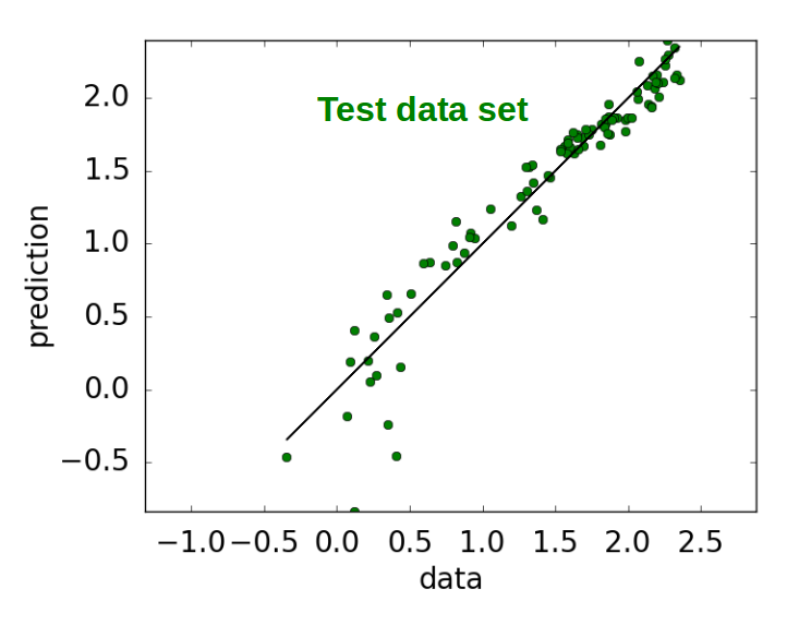
The ability of the model with the lowest squared error to predict the cross validation data set, is then used to predict the test data set, as illustrated below. Each green dot represents a country in a particular year. A perfect model would have all of the points lying along the black line. This model did not use the features of immigration, years women spent in school, and government health spend. The last two features were not required as they are strongly correlated with years men spent in school and total health spend, respectively. In addition the regression coefficients for the features of population, population growth, years men spent in school, GDP and death rate were also orders of magnitude smaller than the coefficients of the dominant features. 

The correlation coefficients of the remaining key features are illustrated below. This indicates that life expectancy is most strongly related to child death rate, with a strong negative correlation of -0.93. This makes sense, since the deaths of very young people would bring down the average life expectancy of the entire country. We also find that the birth rate is higher in countries with higher child death rate, with a strong positive correlation of 0.84. Finally the child death rate is lower in countries with higher health spend per capita, with a negative correlation of -0.4.

When inspecting scatter plots of the key features, the relationship between child death rate and health spend per capita is actually far stronger than the correlation coefficient of -0.4 initially suggests. In the scatter plot highlighted in the figure below you can see there is a very tight arrangement of the samples, with the child death rate dropping rapidly past a threshold health care spend. The relationship is a very strong, but not a linear one, which is why the correlation coefficient was not excessively high. To improve the predictability of the model one could perform a transformation linearising the data prior to undertaking the regression, or adopt a nonlinear regression method such as neural networks. This will be the subject of a future post. For completeness, histogram estimates of the probability density functions are illustrated in the plots along the diagonal of the figure below.

In summary the best way to improve the life expectancy of a country is to reduce the child death rates, which has a very strong relationship to the money spent on health care.

References:

[1] Bengio, Y., Goodfellow, I. J. & Courvill, A., Deep Learning, book in preparation for MIT press, www.iro.umontreal.ca/~bengioy/dlbook

[2] Tibshirani, R. 1996, Regression shrinkage and selection via the lasso, J. Roy. Soc. B., pp267-288.

[3] Ng, A., 2015, Course in Machine Learning, Stanford University, https://class.coursera.org/ml-005/lecture